In the first SPSS tutorial, I touched on the preliminaries of SPSS including the SPSS interface and how to enter data in SPSS.
In this second tutorial, I demonstrate how to manipulate data in SPSS. Data manipulation can take various forms depending on what the researcher wants. This tutorial will cover four main types of data manipulation including: how to categorise data, how to recode a variable, and how to compute a new variable.
This tutorial will use an existing dataset named the Kenya Integrated Household Budget Survey conducted in 2015/2016.
How to categorise data
This manipulation technique is used when you have a continuous variable that you want to categorise into groups.
For example, age in years categorised into age groups, household income amounts categorised into income levels (e.g low-income, middle-income, and high-income) etc.
For this demonstration, the dataset has a variable called household size (hhsize) which refers to total persons in a household, as seen in the image below.
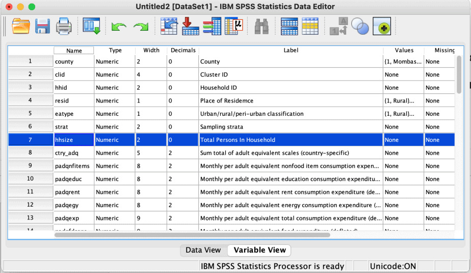
I want to categorise this variable into groups (small, medium and large households).
The steps involved are:
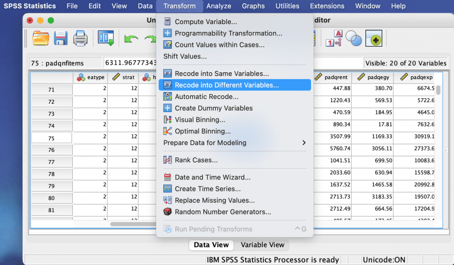
1. Click on Transform menu > recode into different variables (see the image below):
2. From the left pane, select the variable that you want to categorise and click on the arrow to move it to the middle pane. On the right pane, give the name of the new variable, its label (description) and click change, as shown in the images below:
3. The dialogue box that opens helps you define the categories and add their values. In this case, three categories will be created (1=0-3 persons in a household; 2=4-6 persons; and 3=7 and more persons in a household).
- To create the first category, 0-3, choose the option: “Range, lowest through value” and put 3 in the box. In the new value section, put 1. Click add.
- To create the second category, 4-6, choose the option: “Range” and put 4 in the box, “through” and put 6 in the box. In the new value section, put 2. Click add.
- To create the third category, 7 and more, choose the option: Range, value through the highest” and put 7 in the box. In the new value section, put 3. Click add.
- After creating all the categories, click continue.
These steps are shown in the images below:
4. The new variable with the categories will be created. Click the data view to see the new variable and the variable to further define it, for example, to give it value labels. To see the value labels, click on the “value labels” ribbon as shown in the fourth image below.
How to recode variables
This option is used when you want to assign different codes to a categorical or dummy variable.
For instance, if gender is coded “1=male, 2=female” and you want to recode it to “0=male, 1=female” etc.
You can decide to recode into the same variable (this changes the original variable) or into a different variable (this keeps the original variable and creates a new variable, like in the above example).
I always prefer to recode into different variables in order to keep the original data unchanged and in case I would want to use the original variable in future.
In this example, we will use the variable “place of residence” (resid) in the same dataset. This variable has been coded “1=rural, 2=urban).
I want to recode the variable as “0=rural, 1=urban”.
The steps involved are:
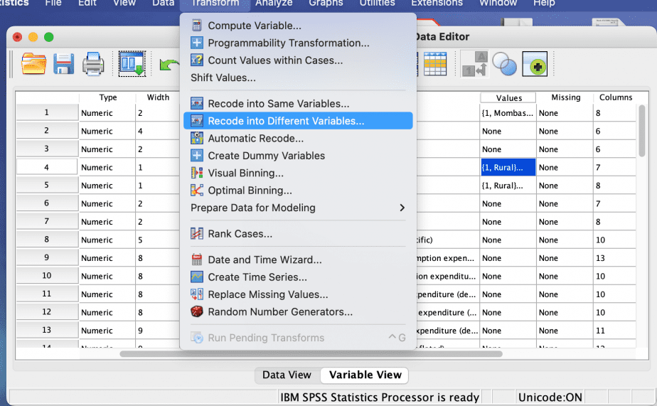
1. Click on Transform menu > recode into different variables (see the image below):
2. Select the variable to be recoded, “place of residence”, and click the arrow to take it to the middle pane.
Name the new variable, in this case I named it “resid_recode” and give it a description in the label box.
Click change.
See the images below:
3. In the dialogue box, put 1 in the old value section and 0 in the new value section. Click add.
This will change the code for rural from 1 to 0.
Similarly, put 2 in the old value section and 1 in the new value section. Click add.
This will change the code for urban from 2 to 1.
Click continue.
See the images below:
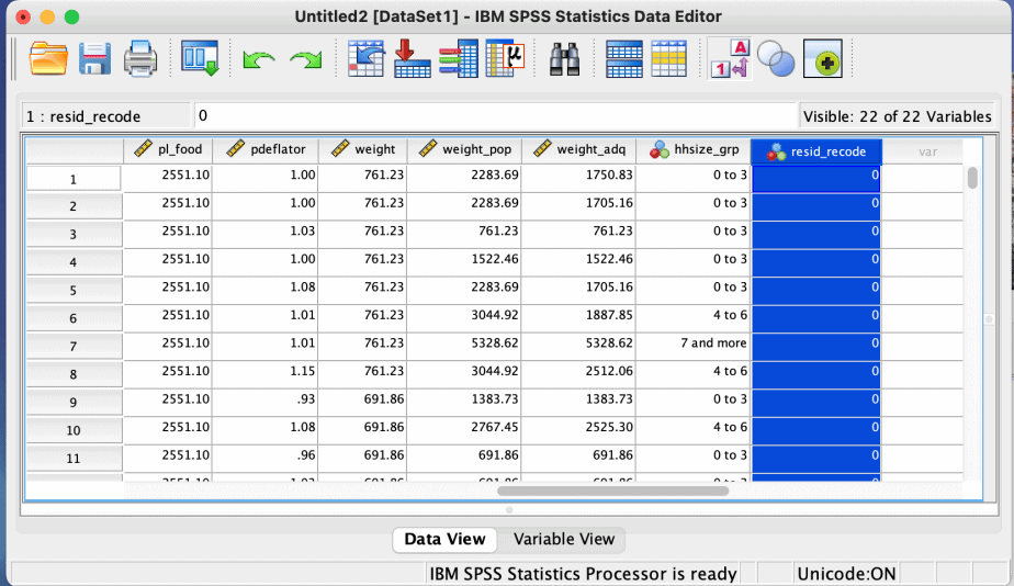
4. The new variable, resid_recode, now appears in the dataset as seen in the data view and variable view.
Use the variable view to further define the new variable, e.g, you can change the decimal places for the variable and add the value labels for the two categories, as shown in the images below:
How to compute a new variable
It is also possible to perform some arithmetics on the data and create new variables using the arithmetics.
For instance, one can be interested in the average of a certain variable, or a ratio between two variables or the total of select variables.
This can be done using the Transform menu as well.
For this demonstration, I am interested in calculating the total monthly household expenditure on some items including: food, education, rent and energy. These variables are named padqfdcons, padqeduc, padqrent and padqegy, respectively.
To get the total monthly household expenditure on these 4 items, I will just sum them together.
The process involves the following steps:
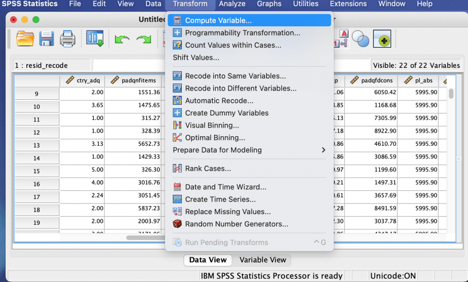
Go to the Transform menu > compute, as shown in the image below:
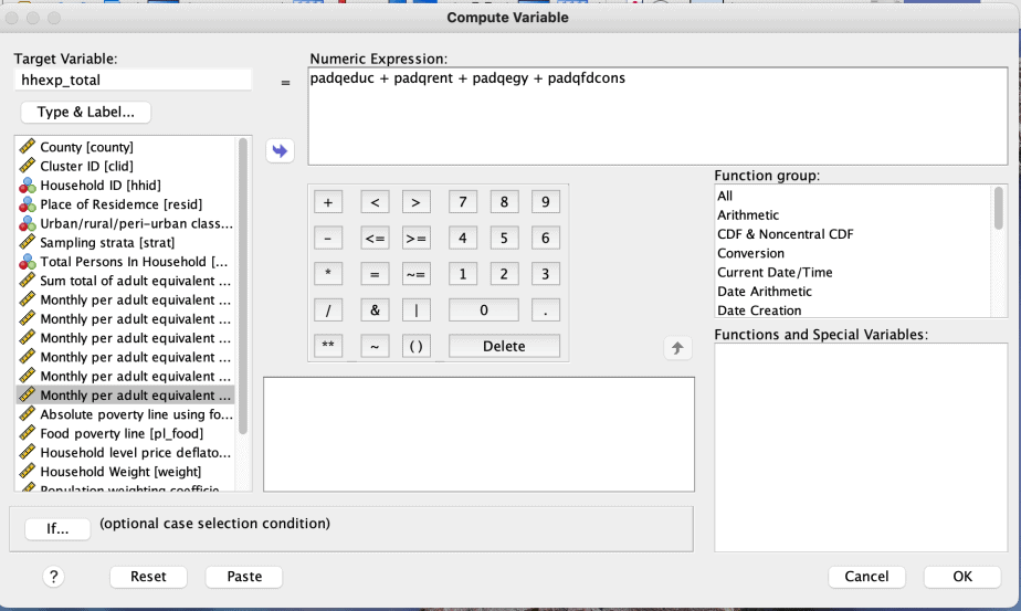
The compute variable window will open.
The compute variable window has several sections:
- Target variable: type the name of the new variable
- Type & Label: specify the type of variable it is and provide a description of the new variable
- Variables list: this section lists all the variables in your dataset. Simply select the variables of interest and use the arrow to put them in numeric expression box.
- Operators: this section has the various arithmetic operators that can be used to compute the new variable.
Perform the arithmetic operation of your interest:
To add the 4 categories of household expenditures, I selected them, used the arrow to put them in the numeric expression box and then used the + sign to add them all together. Alternatively, I could have used the expression “SUM(list of variables) to perform the same operation.
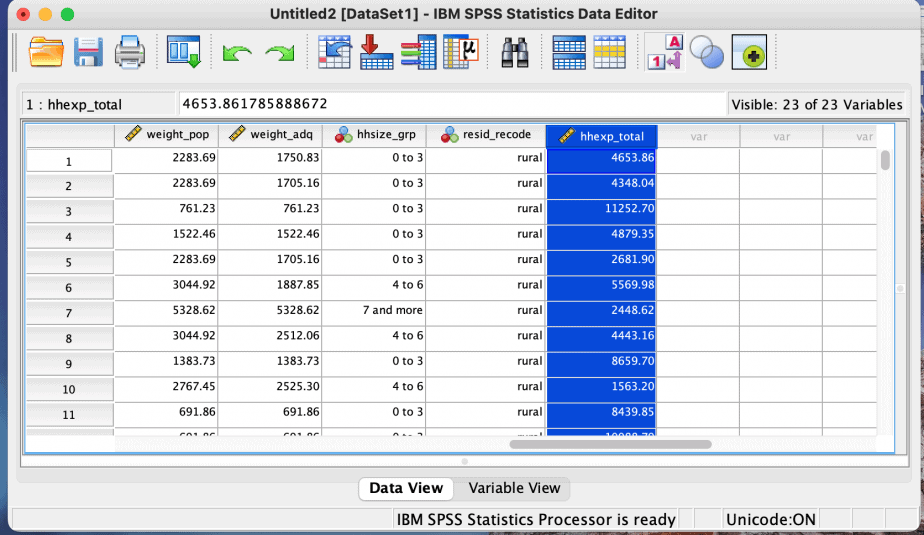
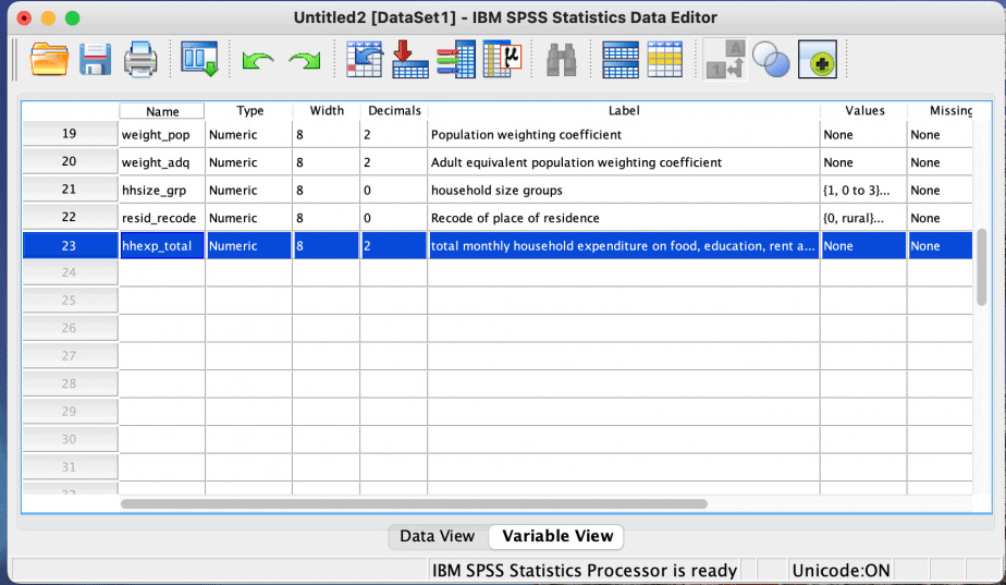
The new variable is created and can be seen in the dataset in both the data view and the variable view, as shown in the images below:
You can further define the new variable in the variable view, if necessary.
In conclusion, a researcher or student can manipulate his data as much as he can and depending on his research needs. SPSS allows data manipulation of different forms. This article demonstrated three common types of data manipulation including: categorisation of data, recoding of variables and computing new variables.
In the next SPSS tutorial, I will cover data modification in SPSS.
Related posts:
How to Code a Questionnaire in SPSS (A Practical Guide)
SPSS Tutorial #1: Introduction to SPSS


