
The normality assumption states that the data is normally distributed. This post touches on the importance of normality of data and illustrates how to check for normality of data in SPSS.
Why is normality of data important?
The normality assumption is important for all parametric tests.
Parametric tests are tests that assume that the parameters of the population from which the sample is drawn are normally distributed.
Examples of parametric tests include: t-tests, analysis of variance (ANOVA), and linear regression.
Characteristics of normal distribution
A normal distribution will have the following key characteristics:
The distribution is symmetrical in appearance, that is, the left side and the right side are almost identical.
The distribution has a bell shape.
The mean, median and mode are almost the same.
Methods for checking normality of data
There are two methods for checking whether a data is normally distributed or not.
These include: graphical methods and numerical (statistical) methods.
Graphical methods
The most common graphs used to check for normality of data include: histogram, box plot, P-P plot, and Q-Q plot.
Numerical methods
The most common numerical/statistical tests used to check for normality of data include: comparing the mean, median and the mode, skewness, the Shapiro-Wilk test, and the Kolmogorov-Smirnov test.
All these tests and graphs can be carried out in SPSS using one command.
How to check for normality of data in SPSS
It is easy to perform both graphical and numerical tests of normality of data in SPSS using only one command: the Explore command.
The procedures are as follows:
Click Analyze > Descriptive Statistics > Explore


The Explore dialogue box will open. Move the variable you want to check for normality into the “Dependent List” box either by dragging-and-dropping or by using the arrow button.
Then click on the “Plots” button.
From the dialogue box, check the options “histogram” and “normality plots with tests.” You may also check the “stem-and-leaf” option.


Click Continue then OK.
SPSS Output
SPSS will produce a number of outputs including statistical/numerical results as well as graphs.
In the example above, we tested for the normality of the variable “age of the respondents”. The outputs produced are as follows:
Output 1: Statistical results
The first output is the descriptive statistics which include: mean, median, skewness, kurtosis, among others.
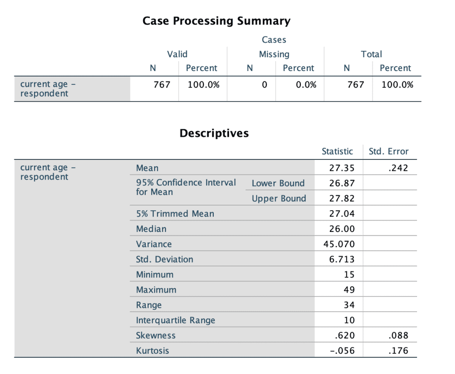
The first output is the descriptive statistics. Compare the mean with the median values to see if they are the same or almost the same. If they are the same, then the data is normally distributed. If they are not the same, then the data is not normally distributed.
Next, check the skewness value. If the value lies between -1 and -0.5, the data is said to be slightly negatively skewed. If the skewness value lies between +1 and 0.5, the data is said to be slightly positively skewed. In the above output, the skewness value is .620, which lies between 0.5 and +1 therefore we can conclude that the data is slightly positively skewed.
Output 2: The Tests of Normality table
The second output produced is the table of Tests of Normality, which gives the results of two tests: the Kolmogorov-Smirnov test and the Shapiro-Wilk test.

Both the Kolmogorov-Smirnov test and the Shapiro-Wilk test have the same null hypothesis, that is, the data is obtained from a normally distributed population. If the Sig. value is less than the p-value (0.05), we reject the null hypothesis. On the other hand, if the Sig. value is greater than the p-value (0.05), we fail to reject the null hypothesis.
From the table of Tests of Normality above, the Sig. value of both tests is less than 0.05. We therefore reject the null hypothesis and conclude that the data is obtained from a non-normal distribution.
The Shapiro-Wilk test is used when the sample size is small (less than 50) but it can also be used for larger samples. The Kolmogorov-Smirnov test on the other hand is more appropriate with a larger sample size. Of the two tests, the Shapiro-Wilk test is said to be more robust than the Kolmogorov-Smirnov test.
Output 3: Histograms
The other output from SPSS is the histogram, which shows how the data is distributed.
Histogram can show whether the data is normally distributed or skewed to the left or right.
Left skew: the tail is towards the left but the data points are concentrated on the right. It is also referred to as positively skewed.
Right skew: the tail is towards the right but the data points are concentrated on the left. It is also referred to as negatively skewed.


From the histograms above, the tail is towards the right and the data points are concentrated on the left. Therefore the data is right (negatively) skewed.
Output 4: Q-Q plots
Besides the histogram, SPSS also produces Q-Q (Quantile-Quantile) plot.


If the data is normally distributed, the data points in the normal Q-Q plot would be concentrated or lie close to the diagonal line. In the above normal Q-Q plot, the data points seem to be straying away from the diagonal line in a non-linear manner, hence we can conclude that the data is not normally distributed.
For the detrended normal Q-Q plot there appears to be an obvious U-shape hence there is a trend of the deviations from the normal. If the data was normally distributed, the deviations would have no obvious trend. We can therefore conclude that the data is not normally distributed.
Conclusion
Testing for normality of a dependent variable is an important step when running parametric tests because these tests assume that the data is normally distributed in the population from which the sample is drawn.
SPSS makes it easy to test for the normality of data by using the “Explore” command which produces both numerical and graphical tests of normality.
If one finds the distribution of the variable to be non-normal, there are two options one can take: either transform the variable (for instance, by calculating the log of that variable) or use non-parametric tests.
Related posts
SPSS Tutorial #9: How to Check for and Deal with Outliers in SPSS