It is rare to have a dataset that is complete hence it is important to know how to code, define and deal with missing data. This is a comprehensive post about missing values in SPSS.
- Reasons for missing data
- Types of missing values in SPSS
- How to code and define missing values in SPSS
- Patterns of missing data
- Missing completely at random (MCAR)
- Missing at random (MAR)
- Missing not at random (MNAR) / Not missing at random (NMAR)
- Missing Value Analysis in SPSS
- Understanding the degree of missing values using descriptives
- Univariate statistics output
- Separate-variance t-tests output
- Cross-tabulations for categorical variables
- Understanding the patterns of missing values in SPSS
- Confirming MCAR using Little’s MCAR test
- How to deal with missing values in SPSS
- Deleting missing values
- List wise deletion
- Pair wise deletion
- Imputing missing values
- Mean substitution
- Imputation using regression
- Imputation using the expectation-maximization (EM) technique
Reasons for missing data
There are many reasons for having missing values/data in a dataset. These include:
Non-applicability of some questions: some questions may not be applicable to some respondents so they leave them blank.
Not knowing the response to some questions: some respondents may lack knowledge about some questions so they will leave them blank.
Refusing to answer: some respondents may know responses to some questions but refuse to answer. This can happen if the question is sensitive or makes the respondents uncomfortable.
Skip logics: in questionnaires with skip logics, there will be missing values if the skip logics require respondents to skip some questions.
Types of missing values in SPSS
SPSS has two types of missing data:
System missing data: these are generated automatically by SPSS. They are denoted with a period mark (full stop) everywhere there are blanks.
User missing data: these are generated by the user/researcher. The researcher will be guided by the codebook used when developing the questionnaire. Common user-generated missing values include 98, 99, 999 etc.
When choosing values to denote missing values, it is important to select codes that are not possible in your dataset. This will vary from one variable to another.
How to code and define missing values in SPSS
As earlier, explained, when choosing codes for missing values, one should select values that are unlikely in the dataset.
To demonstrate, see the examples below of two variables, gender and income level:
| Gender | Income level |
| 1. Male | 1. < $1,000 |
| 2. Female | 2. $1,001 – $3,000 |
| 3. Other | 3. $3,001 – $5,000 |
| 96. Prefer not to say | 4. >$5,000 |
| 96. Not applicable |
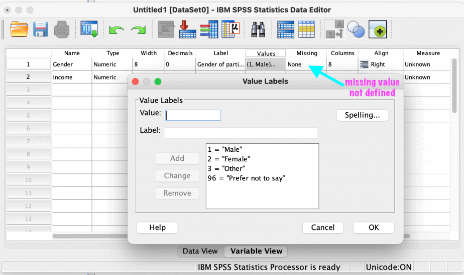
As shown in the table above, the options “prefer not to say” and “not applicable” have been coded 96.
The next step is to define the missing values in SPSS. If this is not done, SPSS will include the 96 values in all the analyses leading to biased results.
To define the missing values in SPSS:
- Open SPSS and create your codebook.
- Go to variable view and select gender.
- Go to the column titled “missing” and click it.
- From the open dialogue box, select the option “discrete missing values” and put in the code “96.” If you have three missing value codes, you can put them in the three boxes. If more than three, you can use the option “range plus one optional missing value.”
- Click OK.
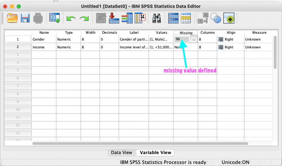
The code “96” will appear in the missing column for that variable.
Repeat the process for all the variables with missing value codes.
This is demonstrated using the gender variable as shown in the images below.
Once you have a dataset that you want to work with, it is important to analyse the missing values to understand the extent of the missing values and the patterns of the missing values.
Patterns of missing data
There are three main patterns of missing data: missing completely at random (MCAR), missing at random (MAR) and missing not at random or not missing at random (MNAR/NMAR).
Missing completely at random (MCAR)
Data are said to be missing completely at random if all the observations have an equal likelihood of being missing.
The missingness is therefore independent of both the observed and unobserved data.
Example: if you are collecting data on students’ performance, but some of the students’ marks got lost, the missing data will be considered as MCAR.
Although considered as a strong assumption, MCAR is often regarded as unrealistic.
Missing at random (MAR)
The second pattern of missing data is the missing at random.
Data are said to be missing at random if there are systematic differences across some groups within the dataset.
The missingness of data in MAR is dependent on the observed data but not the unobserved data.
Example: if you are collecting data on income, and more males than females refuse to provide their income levels, then the missingness of data on income is dependent on gender (observed data), and this is considered to be MAR.
Missing not at random (MNAR) / Not missing at random (NMAR)
Missing not at random or not missing at random occurs when the missing data are dependent on unobserved data that the researcher cannot measure.
Hence the reasons for missing in this case are beyond the knowledge of the researcher.
Example: if you are collecting data on drug abuse in schools, the students who abuse drugs more are unlikely to respond to the survey. Hence the missingness in this case is related to the extent of drug abuse, which the researcher cannot directly observe.
Understanding the patterns of the missing data in a dataset is important because it will guide the researcher on the most appropriate strategies of dealing with the missing data.
Failing to deal with missing data appropriately can lead to biased results.
Missing Value Analysis in SPSS
SPSS has a useful function called the Missing Value Analysis (MVA) that enables a user to analyse the extent and pattern of missing data in a dataset.
Understanding the degree of missing values using descriptives
To use the MVA feature of SPSS, follow the procedure below:
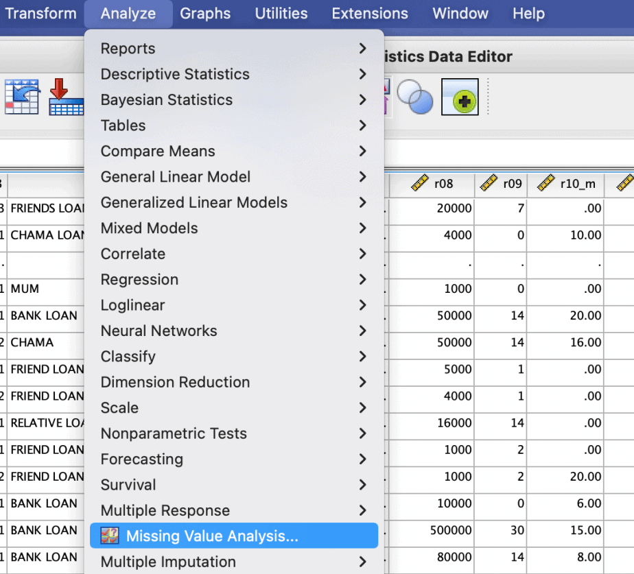
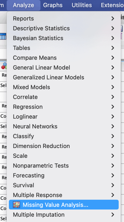
- Click on Analyze menu > Missing Value Analysis
- In the dialogue box that opens, specify the quantitative variables and the categorical variables.
- Click Descriptives:
- The univariate statistics will show the extent of the missing data for each of the listed variables.
- The indicator variable statistics will provide more details about the effects of the pattern of missing data in one variable on the values of other variables.
- The indicator variable refers to data present and data missing for each of the variables.
- Under the indicator variable statistics, select the options “t-tests with groups formed by indicator variables” and “cross tabulations of categorical and indicator variables.
- Click Continue > OK.
The above procedure is demonstrated in the images below:
The procedure will result in three different outputs: univariate statistics, separate-variance t-tests, and cross-tabulations for categorical variables. These are shown below:
Univariate statistics output
The output for univariate statistics looks like the image below:
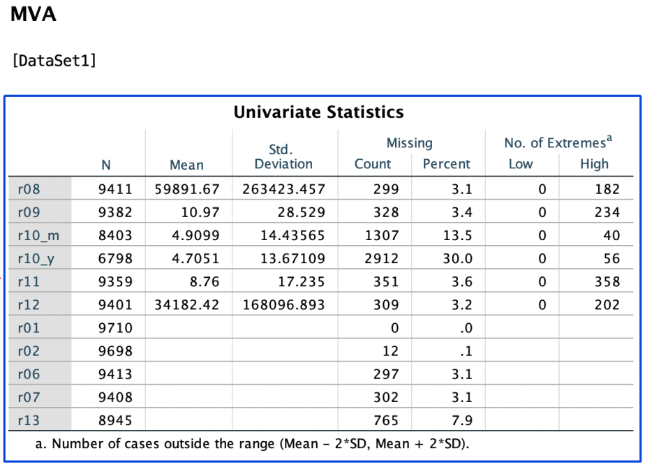
The column N shows the total number of present values for each listed variable.
The column Missing has two parts: count and percent. The count column shows the number of missing values, while the percent column shows the percentage of the missing values for each variable listed.
The recommended percentage of missing values is 5 percent or less. In the table above, variables r10_m, r10_y and r13 have more than the 5% allowable threshold and need to be analysed further using the separate-variance t-tests.
Separate-variance t-tests output
The second output gives the results of the t test conducted for all the quantitative variables using indicator variables with more than 5% missing values.
The output is shown in the image below:
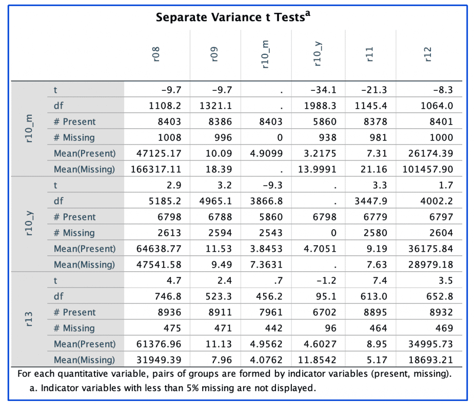
The first column shows the indicator variables for all variables (present vs. missing) with more than 5% missing values (r10_m, r10_y and r13).
In addition to the actual number of missing vs. present values, the means are also displayed.
The first row displays all the quantitative variables.
The table shows how the missingness of one variable affects the values of other variables.
Example: when r10_m is present, the mean value for r08 is 47,125; but when r10_m is missing, the mean value for r08 is 166,317. This is a very big difference and shows that the missingness of r10_m is affecting the mean of r08. This is also the case for all the other quantitative variables.
On the other hand, the missingness of r10_y seems to affect the means of r08, r10_m, and r12.
Lastly, the missingness of r13 seems to affect the means of r08, r10_y, and r12.
Cross-tabulations for categorical variables
The last output is the cross-tabulations for all the categorical variables that were listed.
The cross-tabulations are similar to what is displayed in the separate-variance t-tests tables, except that in this case the categorical variables are displayed instead of the quantitative variables.
The tables also display the frequencies for each indicator in each category in the categorical variables.
Example of cross-tabulation for variable r07 (main reason of obtaining loan) is shown below:

The tables helps one to determine whether there are significant differences in missing values across the various categories of the categorical variable.
Example: missing values for r13 (collateral for credit) are high for the categories “subsistence needs” and “purchase of agricultural machinery” but low for all the other categories.
From the separate-variance t-tests and cross-tabulations, if there are some correlations between variables, it implies that the missing data are missing on random. If there are no correlations, it implies that the missing data are missing completely at random.
Once you have analysed the extent of the missing values and how they affect other variables, it is important to further analyse the patterns of the missing values.
Understanding the patterns of missing values in SPSS
To analyse the patterns of the missing values in SPSS, follow the procedure below:
- Click on Analyze menu > Missing Value Analysis
- Click Patterns
- In the Patterns dialogue box, you can select various patterns tables. Select “tabulated cases, grouped by missing value patterns.” This will also select “sort variables by missing value pattern.
- If you select the option “cases with missing values, sorted by missing value patterns”, you will get a table that lists each case with a missing value and the pattern(s) of the missing values. If your dataset is large, you will get a very long table.
- Click Continue > OK.
The procedure is demonstrated in the image below:
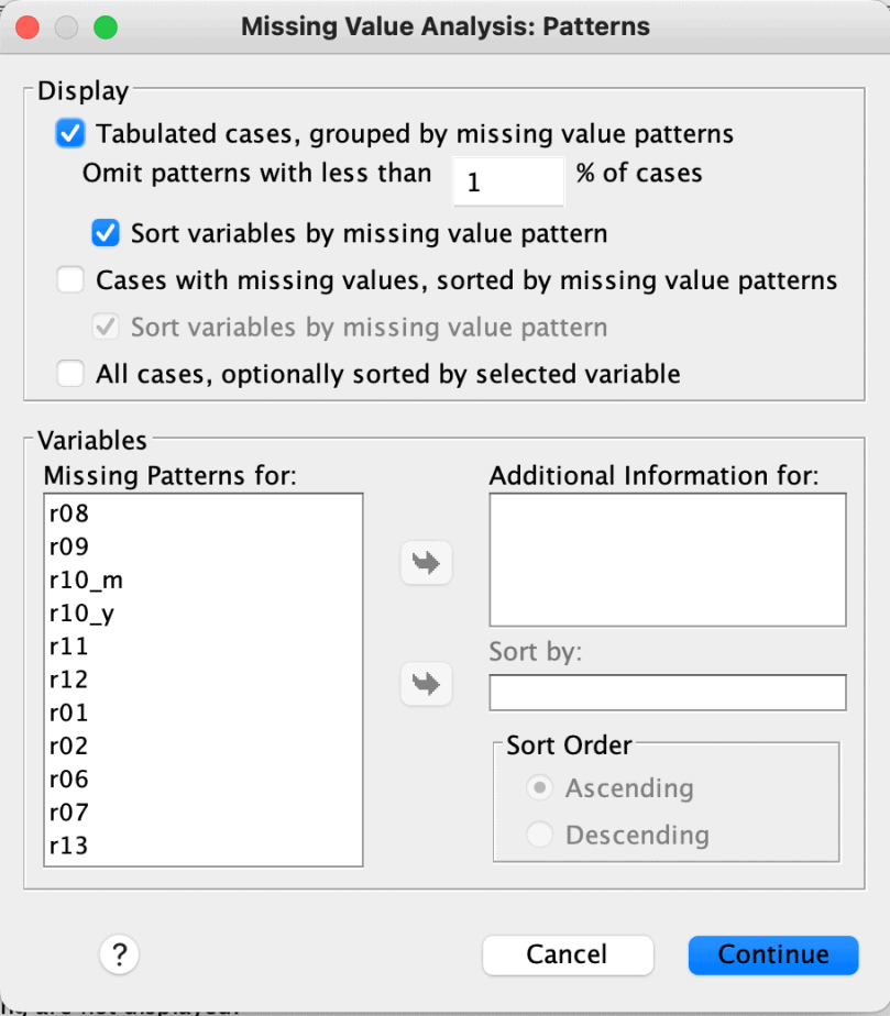
If you found some variables that seem to influence the data, you can include them in the “additional information for” box to get additional information about the variables.
The results from the above procedure are shown below:
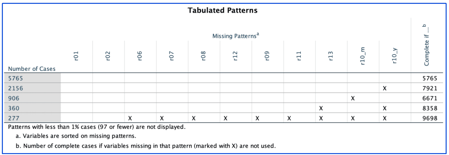
The tabulated patterns table shows that:
- 5765 cases have complete values for the variables listed.
- 2156 cases have missing values for variable r10_y.
- 906 cases have missing values for variable r10_m.
- 360 cases have missing values for variables r13 and r10_y combined.
- 277 cases have missing values for all variables except r01 and r02.
Confirming MCAR using Little’s MCAR test
You can confirm whether the data are missing completely at random using a test called Little’s MCAR test.
This test is also found in the MVA function.
To conduct the test:
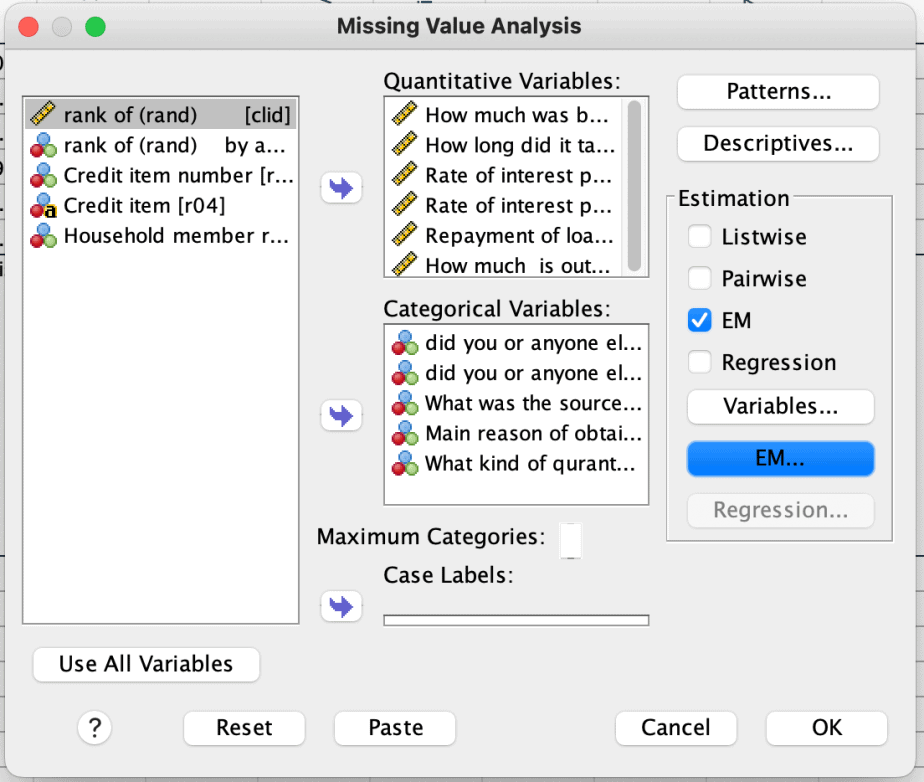
- Click Analyze > Missing Value Analysis
- Click on “EM” under the estimation section > click EM again from the list below
- From the dialogue box that opens, select “normal”
- Click Continue > OK.
The results will be displayed, as shown below:
The null hypothesis of the Little’s MCAR test is that the data are missing completely at random.
This is determined by comparing the significance value with an alpha value of 0.05. If the significance value is less than the alpha value, then the null hypothesis is rejected, and vice versa.
In the example above, the significance value is less than the alpha value of 0.05 so the null hypothesis of MCAR is rejected. The conclusion is that the data are not missing completely at random.
How to deal with missing values in SPSS
After identifying the extent of the missing values and their patterns, the next step is to decide on how to deal with them so that results from data analysis is not biased.
There are two strategies of dealing missing values: deletion and imputation.
Deleting missing values
One can choose to delete missing values if the affected cases are few in number and therefore the sample size will not be significantly reduced.
Additionally, if one or two variables are significantly affected by missing values, you can delete the variables from the dataset.
There are two types of deletion of missing values:
List wise deletion
This strategy deletes all the missing values from the dataset.
A case will be deleted even when it has only missing value.
The analysis will therefore be based on a complete dataset.
This strategy is not recommended as it can significantly reduce the sample size.
Pair wise deletion
It is also known as “exclude cases analysis by analysis”
It deletes cases only if the data missing are required for the analysis being conducted.
This means that the data used will depend on the analysis being conducted and will therefore vary from one analysis to another.
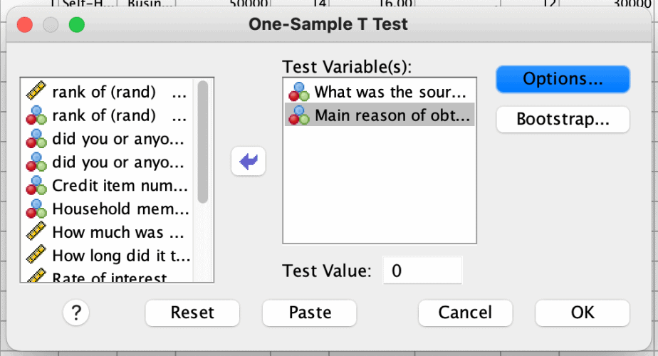
Both deletion methods can be found in SPSS by clicking “options” when running any statistical analysis.
Example: a one sample t-test is conducted as shown below. The “exclude cases analysis by analysis” is selected as the deletion method.
Imputing missing values
The second strategy of dealing with missing values is imputation of the missing values.
There are three ways of imputing missing values:
Mean substitution
In this strategy, the mean of the variable is calculated and all the missing values in that variable are replaced by the mean.
To do this in SPSS:
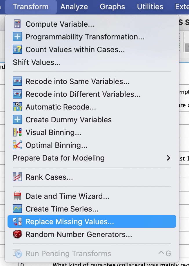
Click Transform > replace missing values
Select the variable of interest. A new variable will be created with a new name.
The method to be used is “series mean.”
Click OK.
All the missing values will be replaced with the mean.
This procedure is demonstrated in the images below:
Imputation using regression
In this method, the missing values are replaced by the predicted value generated from multiple regression.
To do this in SPSS:
Click Analyze > Missing Value Analysis
Specify the quantitative variables and select regression under the estimation options.
In the variables option, you can either specify the predicted and predictor variables, or you can use all the quantitative variables.
In the regression dialogue box, select residuals as the estimation adjustment.
Select the option “create a new dataset” and specify the name of the new dataset. This will ensure that the original dataset remains unchanged for future use.
Click Continue > OK.
This is demonstrated in the images below:
A new dataset will be created with complete data.
Imputation using the expectation-maximization (EM) technique
In this method, the missing data are first imputed using regression analysis.
The complete data with the imputed data is then estimated using maximum likelihood.
To do this in SPSS:
- Click Analyze > Missing Value Analysis
- Click on “EM” under the estimation section > click EM again from the list belo
- From the dialogue box that opens, select “normal”
- Select the “save complete data” to create a new dataset and specify the name of the new dataset.
- Click Continue > OK.
A new dataset will be created with complete data.
Of the 5 methods of dealing with missing data, the imputation using EM is the most recommended.
In conclusion, this post provides comprehensive information using illustrative images on how to define, analyse and deal with missing values in SPSS. The Missing Value Analysis feature in SPSS has also been discussed and demonstrated with practical examples.


