
Simple linear regression is used to model the influence of one variable, called the independent variable or predictor variable on another variable, called the dependent or outcome variable. In this post, I delve into how to run a simple linear regression in SPSS and how to interpret the results from the analysis.
To run a simple linear regression, the dependent variable must be a continuous variable whereas the independent variable can either be a continuous or discrete variable.
How to run simple linear regression in SPSS
As an illustration, I will run a model that has the age of a woman at first birth as the dependent variable, and education in single years as the independent variable.
The interest is to see if women with more years of education have their first child at a later age compared with women with less years of education.
In SPSS:
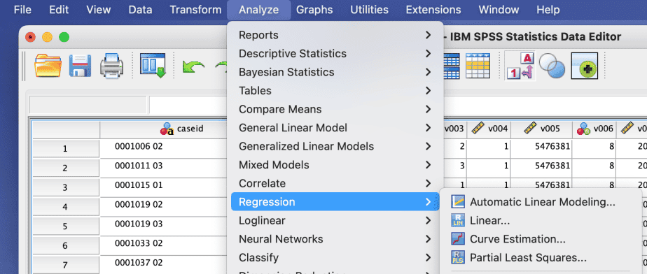
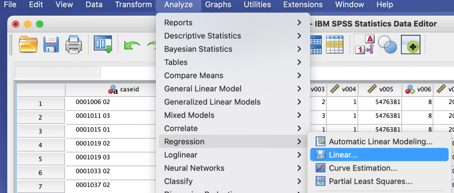
- Go to SPSS menu > Analyze > Regression > Linear
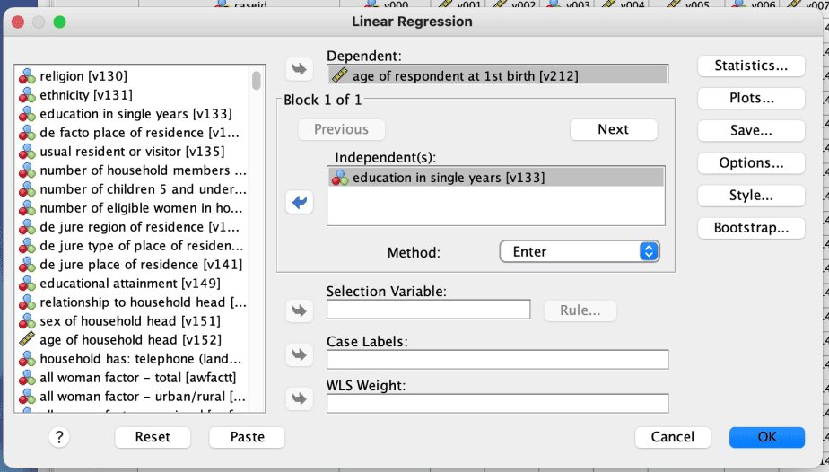
- In the linear regression dialogue box, select the dependent variable of interest and move it to the Dependent: box
- Then select the independent variable and move it to the Independent(s): box
- Click on Statistics

- From the linear regression statistics dialogue box, check the options Estimates and Model fit and click continue then OK
The results displayed will have several parts:
Interpreting the results of simple linear regression in SPSS
a) Variables entered/removed
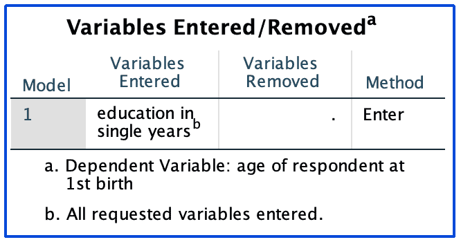
The variables entered/removed table shows:
Which variable was entered in the model as the independent variable and which variable is the dependent variable. In this example, the independent variable is education in single years, whereas the dependent variable is the age of respondent at 1st birth.
The method that was used. In this case, the method used is the Enter method, in which the researcher specifies the variables of interest.
b) Model summary table
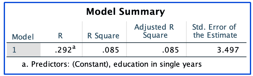
The model summary table shows:
The R, which is the correlation coefficient between the two variables of interest: education in single years and age at 1st birth. In the above example, the R shows that the two variables are positively correlated. However, the magnitude of the correlation coefficient is small, implying a weak correlation between the two variables.
The R Square, which is also referred to as the coefficient of determination. The R square, when converted into a percentage, shows the proportion of variability in the dependent variable that is explained by the independent variable. In the example above, education in single years explains (.085*100=8.5%) only 8.5 percent of the variability in respondents’ age at first birth.
The Adjusted R Square, which is more useful in multiple regression models where many independent variables may be added to the model which are not necessarily useful in explaining the variability in the dependent variable. In simple linear regression models where there is only one independent variable, the Adjusted R Square tends to be the same as the R Square.
The Standard Error of the Estimate.
c) ANOVA table
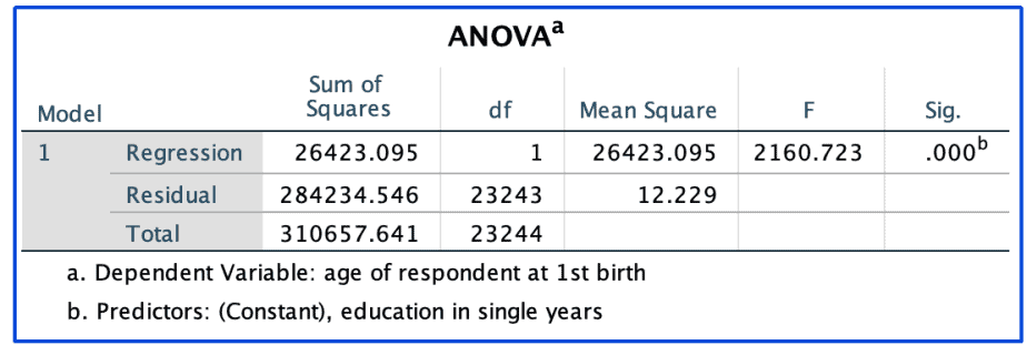
The table displaying ANOVA, which stands for Analysis of Variance, basically divides the total variability in the dependent variable into explained (regression) and unexplained (residual) variability and tests whether there is a difference between these two groups.
If the F-statistic is significant (as shown by the Sig. value), then it implies that the predictor is statistically significant and explains variability in the dependent variable.
d) Coefficients table

The table of coefficients provides the coefficients for both the constant (that is, the value of the dependent variable when the independent variable is equal to zero) and the independent variable.
It also displays both the unstandardized and standaridized coefficients, the standard errors, their t-values and their significance.
In the example above, the coefficient for the constant is 17.605. This implies that for women with no education, their mean age at first birth is approximately 17 years.
The coefficient for education in single years is .252. This implies that an increase in the education of the women by one year increases their age at first birth by .252. This variable is statistically significant as shown by the Sig. value of .000, which is less than an alpha value of .05.
The standardized coefficients are more useful in multiple linear regression models because they enable one to compare which of the independent variables have bigger effects on the dependent variable.
Conclusion
In summary, this post has provided an illustration of how to run a simple linear regression in SPSS along with a practical example of how to both run a simple regression model and how to interpret it. In real-world scenarios, simple linear regression models are rarely used. Instead, multiple regression models are more common.
Related post