In this post, I introduce regression analysis, differentiate between dependent and independent variables, the three sums of square: sum of squares total, sum of squares regression and sum of squares error, as well as the co-efficient of determination. It is the first in a series of posts that will teach regression analysis models and techniques.
- What is regression analysis?
- Regression vs. causation vs. correlation
- Dependent vs. independent variables
- Linear regression model
- Sum of squares total, sum of squares regression and sum of squares error
- Sum of squares total (SST)
- Sum of squares regression (SSR)
- Sum of squares error (SSE)
- Co-efficient of determination
- Population regression function vs. sample regression function
- Hypothesis testing in regression analysis
- Recommended readings
What is regression analysis?
Regression analysis is the most common method used to predict or to make inferences about the relationship between two or more variables.
It is used when a researcher suspects a causal relationship between two or more variables.
The end goal of regression analysis is to predict the population’s average (mean) value of the dependent variable given the independent variables.
Regression vs. causation vs. correlation
Whereas regression deals with the dependence of one variable on another variable(s), it is important to rely on theory to establish whether there is a causation in that relationship.
Assuming two variables, house size and family size, a researcher may be interested to know if one variable causes the other.
Does family size cause house size? Or does house size cause family size?
It is highly possible that when a family size increases, the family is likely to move into a bigger house. Therefore, family size is highly likely to cause house size.
Correlation analysis on the other hand looks at whether the variables of interest have some sort of association, the direction of that association and the strength of that association.
In the example above, it is highly likely that house size and family size have a positive association.
However, correlation does not always imply causation. It is highly unlikely that house size would cause family size.
In correlation analysis, there is no dependent and independent variable, both are treated the same: correlation between family size and house size is the same as the correlation between house size and family size.
Dependent vs. independent variables
It is important to distinguish between the dependent variable and the independent variables in regression analysis for the following reasons:
- It helps a researcher to design his regression model
- It also determines which regression analysis model the researcher will use: there are different types of regression models. Knowing which model to use is important for any researcher.
A dependent variable is the variable that the researcher wants to predict from the model.
It is also referred to as the predictand, explained, regressand, response, endogenous, outcome and controlled variable.
It is denoted as Y.
The dependent variable in regression analysis is always assumed to be random (stochastic) and has a probability distribution.
An independent variable on the other hand is the variable that causes the dependent variable to change.
It is also referred to as the predictor, explanatory, regressor, stimulus, exogenous, covariate, or control variable.
It is denoted as X.
The independent variable in regression analysis is always assumed to be fixed (non-random/non-stochastic).
For every fixed level of the independent variable, there are random values of the dependent variable.
The dependent variable is therefore a function of the independent variable, as shown in equation 1 below:

Linear regression model
The function in equation 1 can take various forms including linear and non-linear.
In regression analysis, we assume that Y is a linear function of X, hence the term linear regression. However, linearity in regression analysis refers to the co-efficients only, not the independent variables. The independent variables can be linear or non-linear.
A linear regression model approximates the causal relationship between Y and X in a linear manner.
The simplest linear regression has only one dependent variable and one independent variable. This model is known as the simple linear regression model.
It is specified as follows in equation 2:

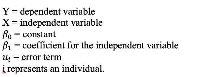
Where:

The constant is interpreted as the value of Y when the independent variable is zero.
The coefficient is interpreted as the change in Y when X changes by one unit, holding other factors constant.
The sign of the coefficient is important: if the sign is positive, it means that if X increases by one unit, then Y will increase by the coefficient. On the other hand, if the sign is negative, it means that if X increases by one unit, then Y will decrease by the coefficient.
The error term is also referred to as the disturbance term or the random stochastic variable and represents all those variables that affect the dependent variable but which were not included in the model.
For linear regression models, the dependent variable must be a continuous variable. The independent variables can be continuous or not.
If the dependent variable is not continuous, then we use other models. for instance, if the dependent variable is categorical, we use the logit/probit models; if it is a count variable then we use the count models.
Besides the simple linear regression model, we also have the multiple linear regression model, where the dependent variable is modelled against two or more independent variables.
Sum of squares total, sum of squares regression and sum of squares error
There are three terms that are important to know and understand in regression analysis:
Sum of squares total (SST)
Also referred to as the total sum of squares (TSS).
It shows the total variability of the dataset; that is, how the observed values differ from their mean values.
It is obtained by squaring the differences between the observed values of the dependent variable and its mean and summing the differences, as shown in formula 3 below:

Sum of squares regression (SSR)
Also referred to as explained sum of squares (ESS).
It shows the explained variability, that is, how well the regression line fits the data.
It is obtained by squaring the differences between the predicted values of the dependent variable and its mean and summing the differences, as shown in formula 4 below:

Sum of squares error (SSE)
Also referred to as residual sum of squares (RSS).
It shows the unexplained (residual) variability.
It is obtained by squaring the differences between the observed values of the dependent variable and the predicted values and summing the differences, as shown in formula 5 below:

The smaller the error, the better the estimation of the regression model.
In regression analysis, the aim is to minimise the error, hence the phrase ordinary least squares (OLS), which is the technique used in linear regression analysis.
The three sums of squares are related in the following way:
SST = SSR + SSE
That is, the total variability of a model = explained variability + unexplained (residual) variability.
Co-efficient of determination
The co-efficient of determination, also referred to as R-squared is obtained by dividing the explained variability of a model (SSR/ESS) by the total variability of the model (SST/TSS), as shown in formula 6 below:

It measures how well the model fits with the data (goodness of fit of the model); that is, the proportion of the variability in the dependent variable that is explained by the independent variables included in the model.
The value of R2 lies between 0 and 1. An R2 of 0 means that none of the independent variables in the model explains variation in the dependent variable. On the other hand, an R2 of 1 means that the independent variables in the model, taken as a whole, explain all the variation in the dependent variable. It is rare to attain an R2 of 1.
Generally, the more the independent variables in a model, the higher the value of R2. However, it is not always the case that as you add more independent variables the R2 will also increase. The variables must be relevant in explaining variation in the dependent variable.
Population regression function vs. sample regression function
It is important to distinguish between a population regression function and a sample regression function:
The population regression function is specified as shown in equation 7:

Where:

The Yi is also interpreted as the expected value of the dependent variable given the independent variables, that is, the average value of the dependent variable in the population given the independent variables.
Because most researchers deal with sample data to estimate the population’s average value of the dependent variable given the independent variables, the researcher’s aim is to estimate the population’s average value of the dependent variable.
The sample regression model is therefore specified as shown in equation 8:

The estimator of Yi is represented as:

Where:

Re-writing equation 8 using equation 9, we get:

The aim of the researcher is to estimate the estimators so that they are as close as possible to the true population parameters.
There are two estimation techniques used in regression analysis, the ordinary least squares (OLS) and the maximum likelihood (ML) techniques. Of these two, the OLS is the most commonly used.
Hypothesis testing in regression analysis
In regression analysis, we use the sample data to make inferences about the population of study.
This is because it is impossible, in most cases, to collect data from the entire population.
In hypothesis testing, we are interested to know if the co-efficients obtained after running the regression model are statistically significant, that is, if they are different from zero.
The hypotheses stated should be based on theories and prior studies.
Recommended readings
Also read:

