In this post, I discuss what correlation is, the two most common types of correlation statistics used (Pearson and Spearman), and how to conduct correlation analysis in SPSS.
What is correlation analysis?
Correlation analysis is used to analyse linear relationships between two variables.
It is mostly concerned with describing the strength and the direction of the relationship.
The strength of a linear relationship: looks at the magnitude of the correlation coefficients. The strength can be small, medium or large.
Correlation coefficients lie between -1 and +1. Ignoring the sign of the coefficient:
- Small correlation: the correlation coefficient lies between .10 and .29
- Medium correlation: the correlation coefficient lies between .30 and .49
- Large correlation: the correlation coefficient lies between .50 and 1.0
The direction of a linear relationship looks at whether the two variables are positively or negatively related.
This is determined by the sign before the correlation coefficient (-1 or +1).
- A positive sign means a positive relationship between the two variables, that is, when one variable increases, the other variable will also increase.
- A negative sign on the other hand indicates a negative relationship between the two variables, that is, when one variable increases, the other variable will decrease.
Types of correlation statistics
There are several types of correlation statistics.
The choice of a correlation statistic should be determined by the level of measurement of your variables.
The two most common correlation statistics are: the Pearson Product-Moment correlation coefficient (denoted as r), and the Spearman rank-order correlation coefficient (denoted as rho).
Pearson correlation
The Pearson correlation (r) is used when the variables are continuous, for instance, the years of schooling in single years and the amount of income.
It is also used when the relationship between the variables is linear, hence, the linearity assumption is an important condition for Pearson correlation.
Spearman correlation
The Spearman correlation (rho) on the other hand is used for ranked or ordinal level data, that is, data that has been ranked in a certain order.
It is also used when the relationship between the variables does not meet the linearity assumption.
It is therefor important to conduct preliminary analysis of the relationship between the variables of interest before conducting correlation analysis. This is best done using the scatterplot.
Preliminary analysis before conducting correlation analysis in SPSS
Before conducting correlation analysis in SPSS, it is important to run a scatterplot for the two variables.
The scatterplot will show:
- whether there are any outliers in your data
- the distribution of the data points: are the data points spread all over the place (indicates little or no correlation), or are they neatly arranged in a particular manner (indicates strong correlation)
- whether it is possible to draw a straight line through the data points (indicates linearity) or whether a curved line is more evident (indicates non-linear relationship)
- the direction of the relationship: if it is possible to draw a straight line through the data points, is the line positively sloped or negatively sloped? This indicates the direction of the relationship between the two variables.
To generate a scatterplot in SPSS:
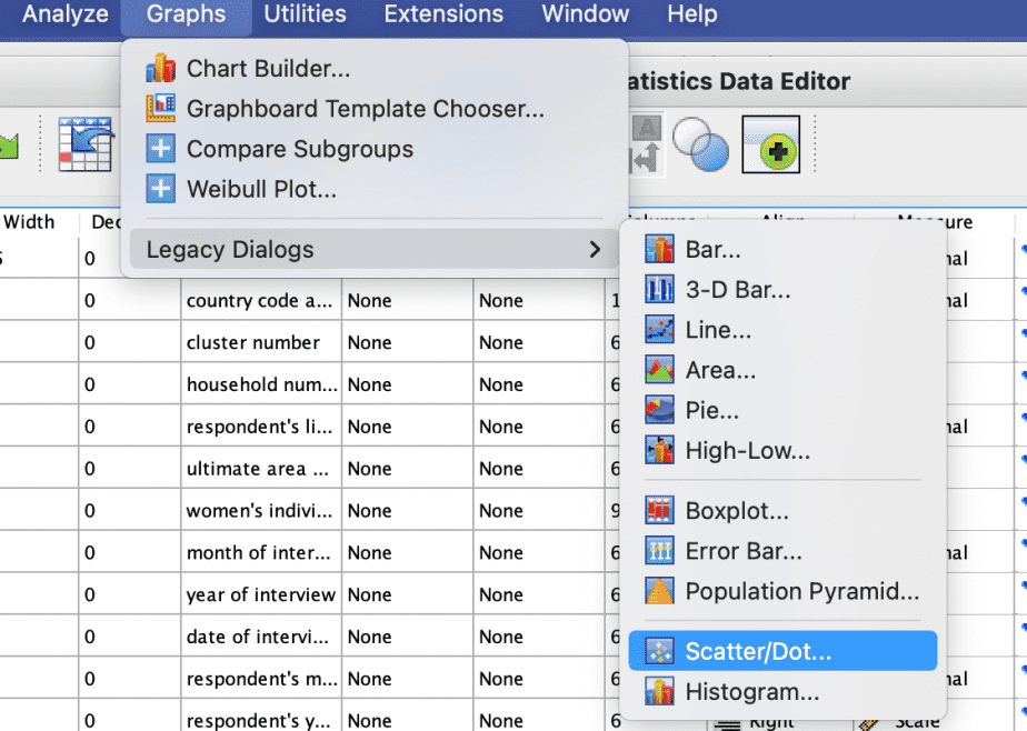
- Click Graphs > Legacy Dialogs > Scatter/Dot
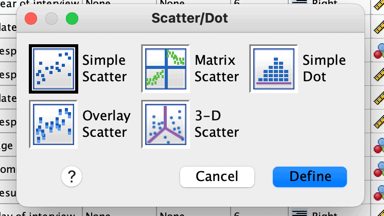
- From the Scatter/Dot dialogue box, select simple scatter then Define
- In the Simple Scatterplot dialogue box, move the dependent variable into the Y axis box, and the independent variable into the X axis box
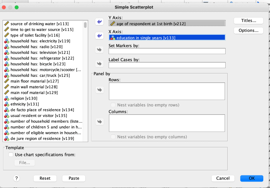
- Click OK.
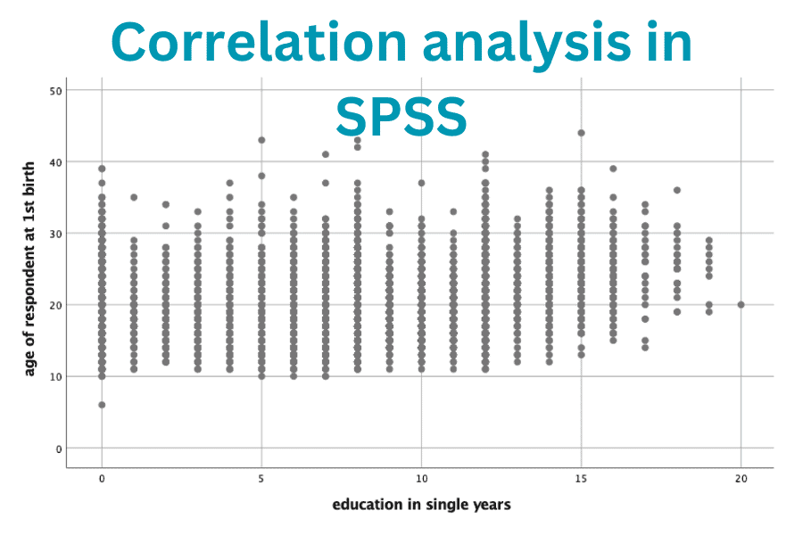
The scatterplot will be generated as shown below:
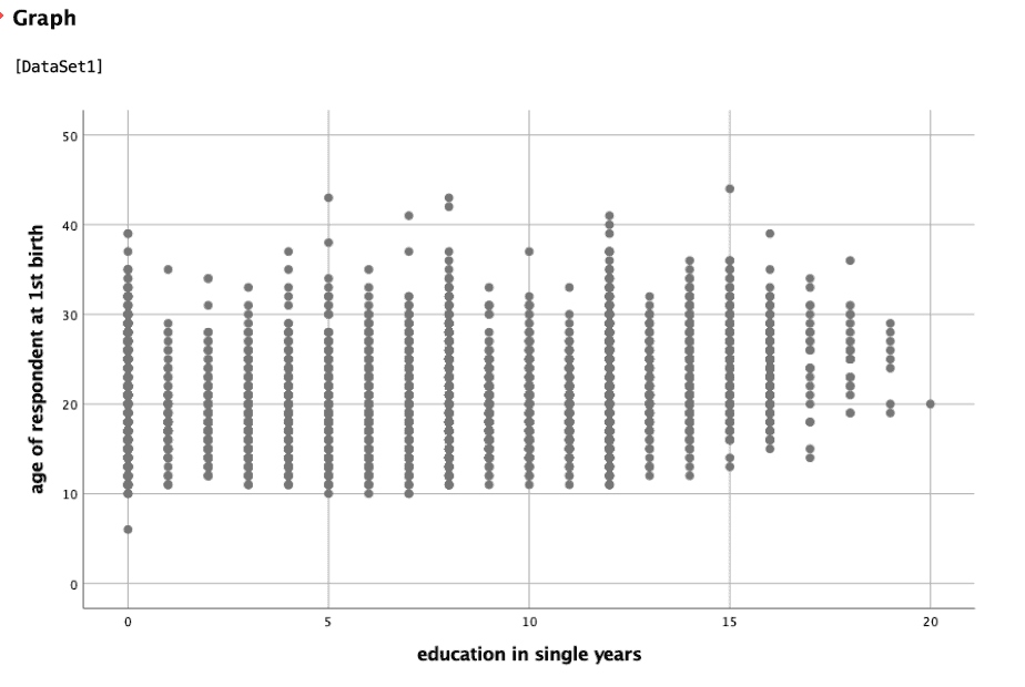
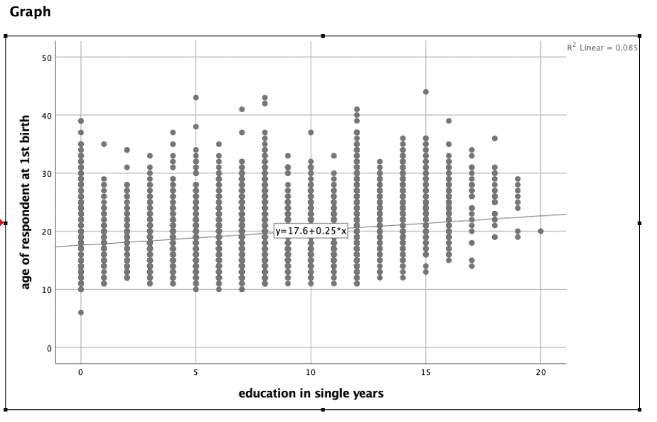
In the example above, we are interested in the correlation between age of respondent (women aged between 15 and 49 years) at 1st birth and education in single years.
The scatterplot shows a positive relationship between the two variables: as the education in single years increases, the age of respondents at 1st birth also increases.
The scatterplot also shows a linear relationship between the two variables, therefore we can go ahead and conduct Pearson correlation analysis in SPSS.
Pearson correlation analysis in SPSS
To perform the Pearson correlation analysis in SPSS:
- Click on Analyze > Correlate > Bivariate
- Select your two variables of interest and move them into the Variables box:

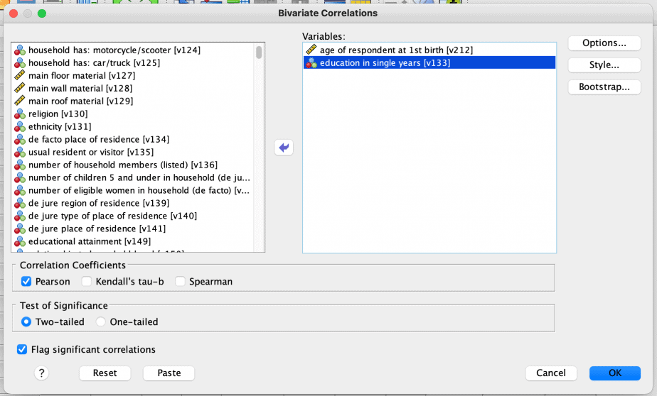
- In the Correlation Coefficients section, check the option “Pearson”
- Click the Options button
- In the Missing Values section, check the option “Exclude Cases pairwise”
- From the Statistics section, you can also check the option “Means and standard deviations” if you wish
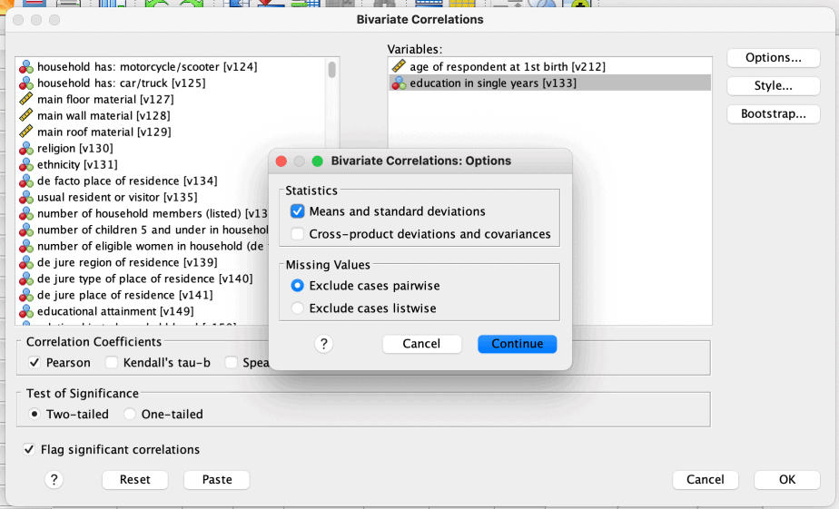
- Click Continue > OK.
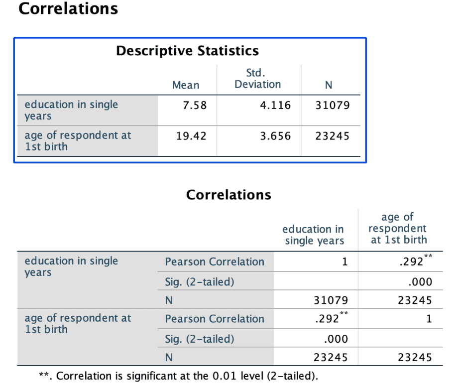
The results will be generated as in the example below:
Spearman correlation analysis in SPSS
To perform the Spearman correlation analysis in SPSS:
- Click on Analyze > Correlate > Bivariate
- Select your two variables of interest and move them into the Variables box
- In the Correlation Coefficients section, check the option “Spearman”
- Click the Options button
- In the Missing Values section, check the option “Exclude Cases pairwise”
- From the Statistics section, you can also check the option “Means and standard deviations” if you wish
- Click Continue > OK.
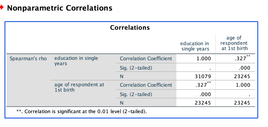
The results will be generated as in the example below. However, for Spearman correlations, the results will be titled “Nonparametric correlations.”
How to interpret the output from Pearson and Spearman correlation analysis
Both Pearson and Spearman correlation coefficients are interpreted in the same manner. There are several things to look for when interpreting the output from the correlation analysis.
The direction of the relationship
As earlier indicated, the direction of the relationship is shown by the sign before the correlation coefficient.
In the outputs above for both Pearson and Spearman correlations, the sign before the coefficients is positive. This implies that the two variables are positively correlated: when education in single years increases, the age of respondents at first birth also increases.
The strength of the relationship
As earlier indicated, the strength of the relationship is indicated by the magnitude of the correlation coefficient.
In the above examples, the Pearson correlation coefficient is .292, which is less than .30. Hence the correlation can be said to be small correlation.
The Spearman correlation coefficient is .327, which is less than .50 hence it can be said to be medium correlation.
The coefficient of determination
Coefficient of determination is used to explain how much one variable explains the variance of the other variable.
It is obtained by squaring the correlation coefficient.
In the above example for Pearson correlation, the coefficient of determination would be (.292)2 = .085.
The coefficient of determination can be turned into percentage for better interpretation. In the example above, the coefficient of determination is .085 X 100 = 8.5%.
This means that the education in single years explains only 8.5% of the variation in age of respondents at first birth.
This implies that there are some other more important factors that explain the variation in age of respondents at first birth.
Coefficient of determination is important when conducting regression analysis.
Assessing the significance level of the correlation coefficient
The significance level is an indication of the level of confidence we should have in the results obtained from the results.
In the above examples, the results are significant at 0.01 level.
Conclusion
This post has discussed correlation analysis, especially the two most common types, that is, Pearson and Spearman correlations. It has also demonstrated how to conduct correlation analysis in SPSS and how to interpret the output from the analysis.

