You have entered your data into Stata. What’s next now? Before you carry out any analysis, it is important to explore and understand your data. This will enable you to perform any required data manipulation before you start your actual data analysis. In this article, I discuss and illustrate various techniques of data exploration in Stata.
Describing data
The describe function or command allows a user to see the properties of the variables in the dataset.
To describe your data, import your data into Stata, go to the Data menu, and select the option Describe data.

Then choose describe data in memory or in a file.
The describe data dialogue box will open. Select the option describe data in memory and click OK.
This option will describe all the variables in the dataset. However, if you are only interested in a few of the variables, specify the variables of interest in the variables box and click OK.

The description of the data will be displayed in the Results window and includes: the variable names, the storage type of each variable, the display format, value labels attached to the categorical variables, and variable labels.
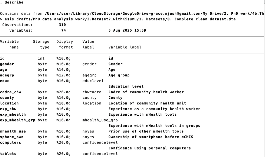
The command syntax for describing data is describe
Summarizing data
You can produce a summary of your data using the summarize feature or command. The summarize action produces a summary of descriptive statistics.
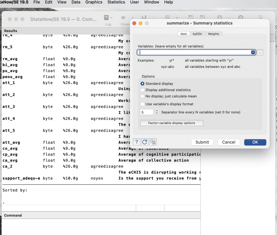
To summarize your data, go to the Data menu and select the option Summary statistics.

The summary statistics dialogue box will open.
You choose to produce summary statistics for all the variables in the dataset, or you can specify the variables of interest.
Click OK.
A table with the summary statistics for each variable will be displayed. The table will include: the number of observations, the mean, the standard deviation, the minimum, andthe maximum values.
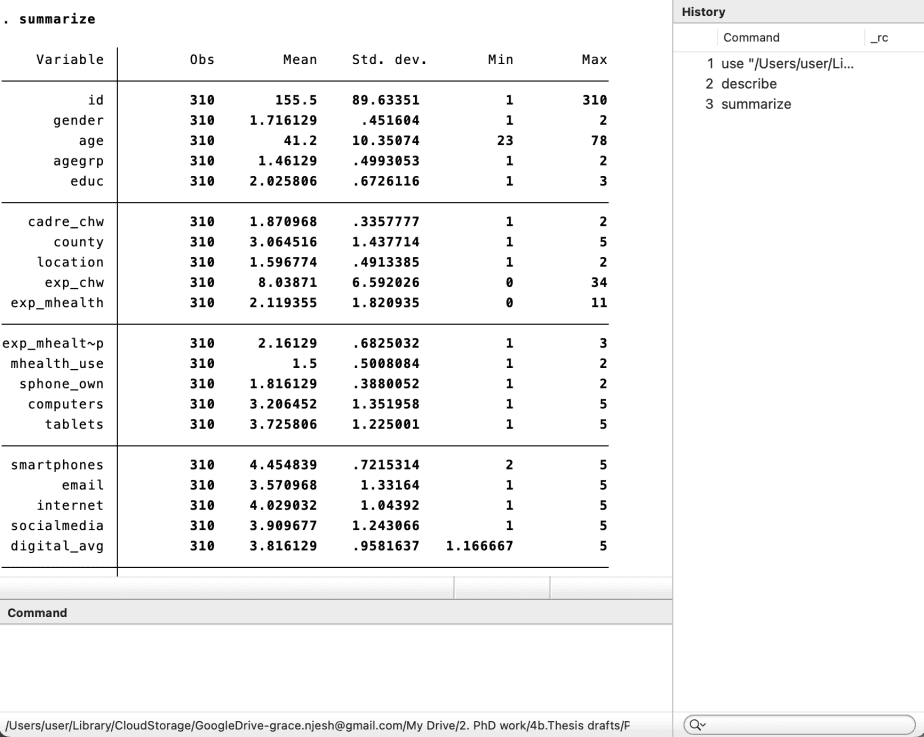
The summary output can help you see if there are variables with missing data, and if the variables are continuous or categorical variables. It will also give you an idea of the variables that are likely to be skewed.
The command syntax for summarizing data is summarize or su in short.
Tabulating data
The summary statistics are more appropriate for continuous variables but not for categorical variables.
To produce summary statistics for categorical variables, the tabulate function is recommended.
You can tabulate individual variables (one-way tabulations) or two variables at the same time (two-way tabulations).
i. One-way tabulations
To produce a one-way tabulation, go to the Statistics menu, then click on Summaries, tables and tests, then Frequency tables.
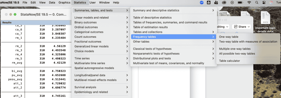
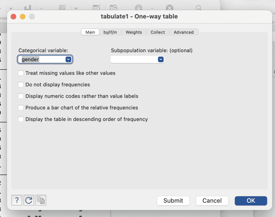
The tabulate-one-way table dialogue box will open. Specify the categorical variable of interest and click OK.
The table of descriptive statistics will be displayed on the Results window.
The descriptive statistics will include frequency, percentage, and cumulative percentage.
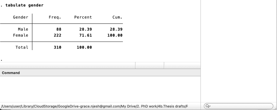
The command syntax for one-way tabulations is tabulate [variable name] e.g tabulate gender.
ii. Two-way tabulations
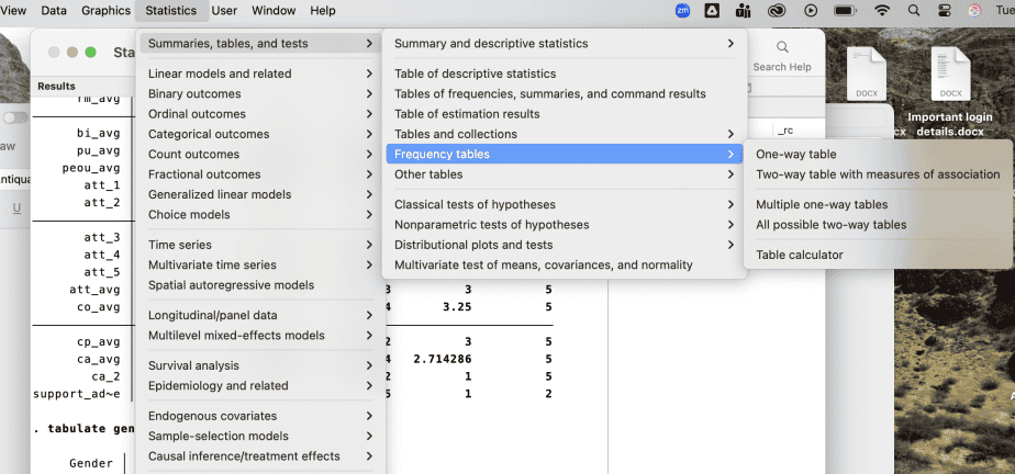
To produce a one-way tabulation, go to the Statistics menu, then click on Summaries, tables and tests, then Frequency tables.
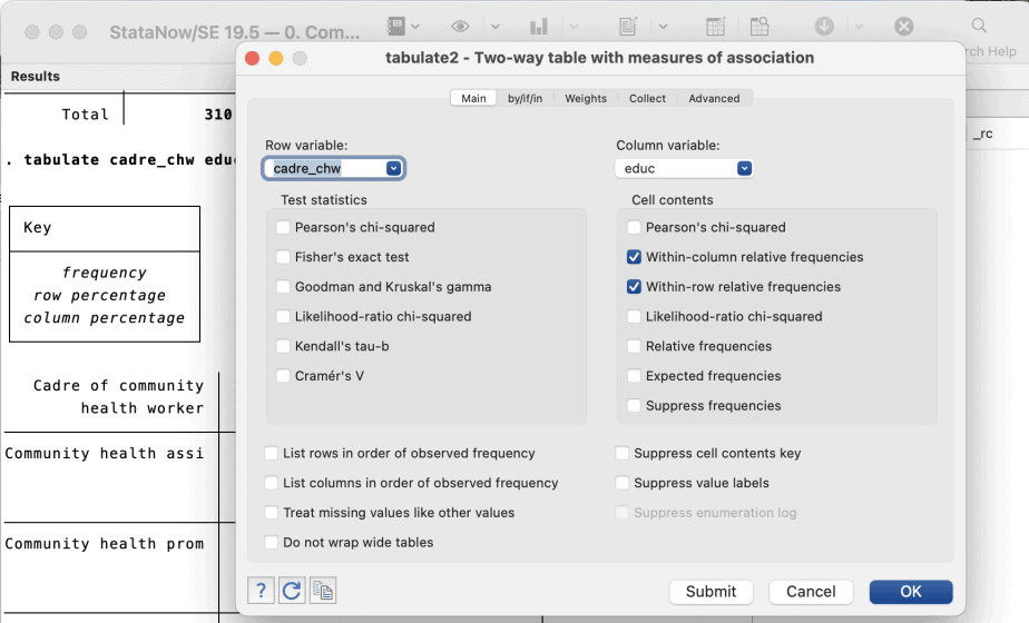
The tabulate-two-way table with measures of association dialogue box will open. Specify the row variable and the column variable of interest. Then select the options “within-column relative frequencies” and “within-row relative frequencies”. Click OK.
The table of descriptive statistics will be displayed on the Results window.
The descriptive statistics will include frequency, row percentage, column percentage, and total frequencies and percentages.
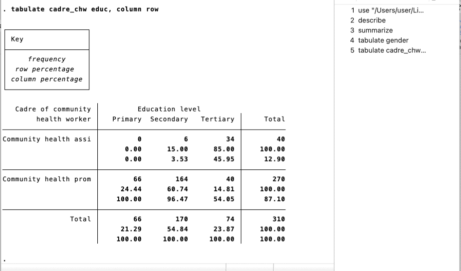
The values on the first row represent the frequencies, the second-row values represent the row percentages, and the third-row values represent the column percentages.
In the output above, we can conclude that:
- There were 40 community health assistants (CHAs) and 270 community health promoters (CHPs)
- Six of the CHAs (15 percent) had secondary-level education, and 34 (85 percent) of the CHAs had tertiary-level education
- Sixty-six of the CHPs (24.4 percent) had primary-level education, 164 of the CHPs (60.7 percent) had secondary-level education, and 40 of the CHPs (14.8 percent) had tertiary-level education
- Sixty-six (100 percent) of those with primary-level education were CHAs
- Six (3.5 percent) and 164 (96.5 percent) of those with secondary education were CHAs and CHPs, respectively
- Thirty-four (46 percent) and 40 (54 percent) of those with tertiary education were CHAs and CHPs, respectively.
The command syntax for producing two-way tabulations with measures of association is: tabulate [variable 1] [variable 2], column row e.g tabulate cadre_chw educ, column row
In conclusion, this post has illustrated various ways of exploring data in Stata, such as how to describe data, summarize data, and tabulate data. Data exploration in State enables one to get a glimpse of the nature of the variables, which in turn informs the need to manipulate some variables before the actual analysis can begin. In the next post, I dive deep into data manipulation in Stata.